Lecture 9: Combining Forecasts
Often there are multiple ways to forecast the same thing, and we’d like a way of combining the forecasts together. For instance, consider the following question:
Will Will be among the top 3 most sold nonfiction books on Amazon for the week of November 21?
(This was posed to the course staff at the beginning of that week.)

I approached this problem using reference class forecasting, but there wasn’t any single very good reference class. Specifically:
- I built up a dataset of the past 6 weeks by manually copying information from the website.
- Will had been #1 last week and #7 two weeks prior (and not released before that).
- 1 out of 3 books in the top 3 remained there the following week (15 data points total).
- 1 out of 5 books in the top 1 were in the top 3 the following week (5 data points total).
- Of books that were top 3 last week and top 8 the previous week, 1 out of 4 stayed in the top 3 (4 points total).
- Of books that were top 1 last week and top 8 the previous week, 1 out of 2 stayed in the top 3 (2 points total).
The problem is that:
- None of these reference classes have many data points.
- The class with the most data points (“top 3 last week”) is the one that’s least analogous to Will.
One way out of this is to combine all the reference classes together in a weighted average. This is called ensembling. I’ll start with a rough intuitive way of doing this and then give a more principled way (as with most things in forecasting, the best approach is to practice the principled way until it informs your intuition, then mostly go with intuitive numbers).
Rough intuitive approach. Let’s give each data source a score out of 10, based on how “good” it seems (a combination of the total number of data points and how analogous it is to Will).
- Top 3: I give this 6 out of 10. There’s a lot of data points but it’s only somewhat analogous.
- Top 1: I give this 3.5 out of 10. More analogous, but few enough data points to have lots of noise.
- Top 3 + top 8: I give this 3 out of 10. Similar to top 1 but one fewer data point.
- Top 1 + top 8: 2 out of 10. Most analogous but no data.
Then we combine as a weighted average: $\frac{6 \cdot (1/3) + 4 \cdot (1/5) + 3.5 \cdot (1/4) + 2 \cdot (1/2)}{6 + 4 + 3.5 + 2} = 0.30$.
More principled approach. The intuitive approach is reasonable, but as written it neglects some obvious information: for instance, the fact that the “top 3” reference class should probably provide a lower bound (since Will was top 1), so we should forecast at least $5/15 = 0.33$ (instead of $0.30$ as above).
We can handle this by more explicitly modeling each of the 4 estimates as “noisy” versions of the true probability. Specifically:
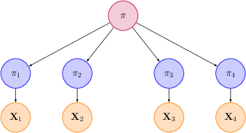
- Let $\pi$ be the “true” probability that Will is top 3 next week.
- For each reference class $i$, let $\pi_i$ denote the probability for that reference class (that is, the fraction of positives we would see if we had an infinite number of samples).
- Finally, let $X_i$ be the observes number of positive samples and $N_i$ the total number of samples for the reference class. So for instance $X_1 = 5$, $N_1 = 15$, and $X_2 = 1$, $N_2 = 5$.
We will think of each $\pi_i$ as a noisy version of $\pi$, and $X_i$ as a noisy version of $\pi_i$:
For instance, if $\pi$ is the probability for Will, I might think the probability $\pi_1$ for a generic top 3 book is somewhere in the range $[\pi-0.2, \pi]$. To model this, I’ll treat $\pi_1$ as a Gaussian with mean $\pi - 0.1$ and variance $0.1^2$.
In general, for each reference class $i$ we might think it has a bias $\Delta_i$ relative to $\pi$, and uncertainty $\sigma_i$, modeling $\pi_i$ as Gaussian with mean $\pi + \Delta_i$ and variance $\sigma_i^2$. Here’s a table of my intuitions for $\Delta_i$ and $\sigma_i$:
| # | Ref. Class | $\Delta_i$ | $\sigma_i$ |
|---|---|---|---|
| 1 | Top 3 | -0.1 | 0.1 |
| 2 | Top 1 | 0 | 0.1 |
| 3 | Top 3 + top 8 | 0 | 0.1 |
| 4 | Top 1 + top 8 | 0 | 0.07 |
(Brief explanation: I intuitively thought “top 1” and “top 3 + top 8” were roughly equally good reference classes for Will, while “top 1 + top 8” was a bit better, so I gave the last one lower $\sigma_i$.)
Going from $\pi_i$ to $\pi$. If we knew $\pi_1, \ldots, \pi_4$, then it turns out that the maximum likelihood estimate for $\pi$ is
$\frac{(\pi_1 - \Delta_1) / \sigma_1^2 + (\pi_2 - \Delta_2) / \sigma_2^2 + (\pi_3 - \Delta_3) / \sigma_3^2 + (\pi_4 - \Delta_4) / \sigma_4^2}{1/\sigma_1^2 + 1/\sigma_2^2 + 1/\sigma_3^2 + 1/\sigma_4^2}$.
In other words, we first correct each $\pi_i$ for its bias, then take a weighted average, weighted by the inverse of the variance. This recovers the weighting idea from the rough intuitive approach. The main advantage is that it gives us a more principled way to think about the weights $1/\sigma_i^2$.
Incorporating sample noise. However, there are still some problems. First, we don’t actually know $\pi_i$: only $X_i$ and $N_i$. We can approximate $\pi_i$ as $\hat{\pi}_i = X_i / N_i$, but we also need to adjust $\sigma_i$. For instance, the table above has $\sigma_4$ as the smallest, meaning we would rely on it most in our average, but that reference class only has $2$ data points.
Fortunately, there is a simple mathematical correction for the difference between $\hat{\pi}_i$ and $\pi_i$. It relies on the assumption that $\hat{\pi}_i$ is an average of independent random variables (the different members of the reference class) and so can be well-approximated by a Gaussian distribution. A standard estimate of the variance of this Gaussian is $\frac{\hat{\pi}_i(1-\hat{\pi}_i)}{N_i-1}$, so we can replace the old $\sigma_i$ with the corrected values
$\overline{\sigma}\_i^2 = \sigma_i^2 + \frac{\hat{\pi}\_i(1 - \hat{\pi}\_i)}{N_i - 1}$
The following table summarizes these calculations:
| # | Ref. Class | $\Delta_i$ | $\sigma_i$ | $X_i$ | $N_i$ | $\hat{\pi}_i$ | $\overline{\sigma}_i^2$ |
|---|---|---|---|---|---|---|---|
| 1 | Top 3 | -0.1 | 0.1 | 5 | 15 | 0.33 | $0.1^2 + 0.016 = 0.026$ |
| 2 | Top 1 | 0 | 0.1 | 1 | 5 | 0.2 | $0.1^2 + 0.04 = 0.05$ |
| 3 | Top 3 + top 8 | 0 | 0.1 | 1 | 4 | 0.25 | $0.1^2 + 0.063 = 0.073$ |
| 4 | Top 1 + top 8 | 0 | 0.07 | 1 | 2 | 0.5 | $0.07^2 + 0.25 = 0.255$ |
Weighting the $\pi_i - \Delta_i$ by $1/\overline{\sigma}_i^2$, we get an overall estimate of $0.34$, which makes more sense than the $0.30$ forecast from before.
Combining the approaches. In practice, it’s probably not worth exhaustively doing the math above to compute $\overline{\sigma}_i$. Instead, I would in fact pick the weights based on intuition, but keep in mind that they are based on two terms: one capturing how similar the reference class is to what we care about (after correcting for bias), and one capturing finite sample error, which decreases at a rate of roughly $1/N_i$.
There are two reasons that computing the weights intuitively, rather than mathematically, is usually better. The first is that the math above depends on independence assumptions that might not hold. For instance, since the “top 1” reference class is a subset of the “top 3” reference class, they are positively correlated, so I’d want to decrease the weight for “top 1” a bit since it’s redundant information. After I did this, my intuitive forecast was $0.36$ rather than $0.34$.
Another important reason is that it’s easy to get caught up in these calculations, when it’s often better to instead look at the problem from additional angles. For instance, one of the other course staff realized that autobiographies often stay in the top 3 for a while, and that Will had so far been particularly well-received within this genre, so gave a probability significantly above 50% (and ended up being right).
Combining External Forecasts
We used the ideas above to aggregate different reference classes, but we can apply the same strategy of averaging predictions whenever there are multiple ways of approaching a forecasting problem.
More interestingly, we can combine predictions of different forecasters. Let’s say that Frances and I both make forecasts about something, but I know that so far she’s had a somewhat better track record than me. Then I could probably do better than either of us by averaging our forecasts but giving hers a 3:1 weight relative to mine. (Or if she’s done much better than me, 10:1; or 1:1 if we’ve done similarly.) You can also do this for larger teams and even for people you don’t know, as long as you have a rough sense of how much to trust them.
In practice, this is how I form beliefs for most topics: I identify a set of experts who have a good track record, and take a weighted average of their views. For a much smaller set of topics, I also develop my own deep “inside view”, although if I were making forecasts I would still average that view with other experts.
However, when practicing forecasting, you don’t want to just defer to others’ forecasts all the time, since then you won’t improve your own forecasting skills. You want to practice both the skill of generating your own forecasts and weighing the forecasts of others. In addition, if you are on a team of forecasters, often the most successful method is the Delphi method, where forecasters first generate predictions individually, then discuss, then generate new predictions and take the average. You’ll get to practice this a lot in the group discussions this semester to get a sense for it.
Summary
Ensembling–the idea of taking weighted averages of forecasts–is a powerful tool for improving over any individual forecast. When assigning weights, you want to consider both the quality of the underlying data and how closely the forecast captures the situation at hand. However, obsessing too much about how to ensemble can also distract you from searching for new information that significantly alters your view—so it’s usually best to perform as a lightweight “post-processing” step.